Calculating Eigenvectors Made Easy
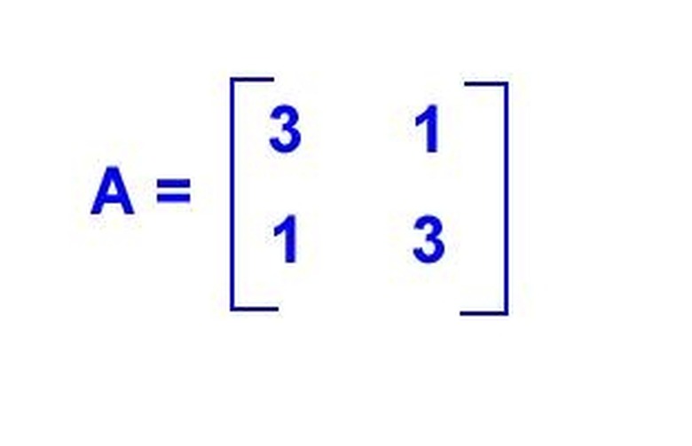
Table of Contents
- Theoretical Background of Eigenvectors
- What are Eigenvectors?
- Role of Eigenvectors in Linear Transformations
- Mathematical Notations and Formulas
- Properties and Behavior of Eigenvectors
- Methods for Finding Eigenvectors
- The Power Method
- Mathematical Formulation
- Advantages and Limitations
- Inverse Power Method
- Mathematical Formulation
- Advantages and Limitations
- QR Algorithm
- Mathematical Formulation
- Advantages and Limitations
- Computational Techniques for Large Matrices
- Iterative Techniques: Arnoldi Iteration
- Restarting and Deflation
- Dense Matrix Compression
- Parallelization
- Numerical Stability and Precision Issues
- Round-Off Error, How to calculate eigenvectors
- Overflow
- Conditioning
- Adjusting Numerical Methods
- Choosing Data Types
- Using Advanced Numerical Libraries or Frameworks
- Applications of Eigenvectors in Various Fields: How To Calculate Eigenvectors
- In Physics and Engineering
- In Data Analysis and Machine Learning
- In Economics and Finance
- In Biology and Medicine
- Eigenvector Properties and Interpretable
- Orthogonality of Eigenvectors
- Eigenvalue Equation Derivation
- Eigenspace Decomposition
- Examples of Interpretable Eigenvectors
- Example 1: Principal Component Analysis (PCA)
- Example 2: Image Compression
- Example 3: Network Community Detection
- End of Discussion
- Clarifying Questions
How to calculate eigenvectors takes centre stage, this opening passage beckons readers into a world crafted with good knowledge, ensuring a reading experience that is both absorbing and distinctly original.
Eigenvectors are vectors that, when a linear transformation is applied to them, result in a scaled version of themselves. This is where the magic happens, folks!
Theoretical Background of Eigenvectors
Eigenvectors are a fundamental concept in linear algebra, and their significance extends far beyond the realm of mathematics. They play a crucial role in understanding the behavior of linear transformations in vector spaces, which has numerous applications in physics, engineering, computer science, and other fields. In essence, eigenvectors provide a way to diagonalize matrices, simplifying complex mathematical operations and revealing the underlying structure of the transformations they represent.
What are Eigenvectors?
A scalar (also known as an eigenvalue) and a non-zero vector (known as an eigenvector) are said to be in an eigenrelation with the linear transformation TA, in the equation: T(v) = λv, where v is the eigenvector, λ is the eigenvalue and T is the linear operator.
In this equation, λ is the scalar that the transformation compresses or stretches, and v is the vector on which this transformation is applied. The eigenvector v can be thought of as the direction in which the transformation TA acts multiplicatively with respect to the scalar λ, and this relationship holds true for all values of λ that satisfy the equation T(v) = λv.
Eigenvectors have the unique property that they are unchanged by the action of the linear transformation except for a possible scale factor. This means that if v is an eigenvector of T with eigenvalue λ, then T(v) = λv, and since v ≠ 0, we can solve for λ as λ = (1/v)T(v). However, the eigenvectors of a matrix are not necessarily unique; in general, there can be many different eigenvectors corresponding to a single eigenvalue.
Role of Eigenvectors in Linear Transformations
Eigenvectors are essential in understanding the behavior of linear transformations, as they reveal the structure of the transformation and provide a basis for diagonalizing the matrix representation of the transformation.In the context of linear transformations, eigenvectors are used to decompose the transformation into a set of simpler transformations, each corresponding to a particular eigenvalue and eigenvector pair. This decomposition is known as the eigendecomposition of the transformation.
The eigendecomposition of a transformation has several important applications in linear algebra, including:
Mathematical Notations and Formulas
The concept of eigenvectors can be expressed using a range of mathematical notations and formulas, which are essential for defining and manipulating eigenvectors in different mathematical contexts. The most common notations and formulas include:Properties and Behavior of Eigenvectors
Eigenvectors have several important properties and behave in distinct ways, which are crucial for understanding their role in linear transformations and for using them in different mathematical contexts. The key properties and behaviors of eigenvectors include:Methods for Finding Eigenvectors
Finding eigenvectors is a fundamental problem in linear algebra and has numerous applications in various fields, including physics, engineering, and computer science. The main goal of this section is to describe different methods used to find eigenvectors, including their strengths and limitations.The Power Method
The power method is an iterative technique used to find the dominant eigenvector of a square matrix. The method starts with an arbitrary initial vector and repeatedly multiplies it by the matrix, normalizing the result at each step. The process is continued until the vector converges to the dominant eigenvector.Mathematical Formulation
vi+1 = A vi
where A is the square matrix, vi is the initial vector, and vi+1 is the result after each iteration.Advantages and Limitations
The power method has the advantage of being simple to implement and compute efficiently, especially for large matrices. However, it has the limitation of requiring an initial vector that is close to the dominant eigenvector, or it may converge to a spurious solution.
Inverse Power Method
The inverse power method is a variation of the power method used to find eigenvectors with small eigenvalues. The method involves multiplying the matrix by its inverse and then applying the power method as described above.Mathematical Formulation
vi+1 = (A-1)vi
where A is the square matrix, vi is the initial vector, and vi+1 is the result after each iteration.Advantages and Limitations
The inverse power method has the advantage of being able to handle large eigenvalues and is often used for finding eigenvectors with small eigenvalues. However, it requires the matrix to be invertible, and numerical instability may arise if the matrix is ill-conditioned.
QR Algorithm
The QR algorithm is a method used to compute eigenvalues and eigenvectors of a matrix. The algorithm involves the QR decomposition of the matrix, which is then updated iteratively to convergence.Mathematical Formulation
A = QR
where A is the square matrix, Q is the orthogonal matrix, and R is the upper triangular matrix.Advantages and Limitations
The QR algorithm has the advantage of being numerically stable and able to handle large matrices. However, it requires careful tuning of the algorithm parameters and may be computationally intensive.
Computational Techniques for Large Matrices
Computing eigenvectors for large matrices using traditional methods can be computationally challenging and time-consuming. As the size of the matrix increases, the number of operations required to compute the eigenvectors grows exponentially, making it impractical to use traditional methods. Modern algorithms have been developed to address these challenges, enabling efficient computation of eigenvectors for large matrices.Iterative Techniques: Arnoldi Iteration
The Arnoldi iteration is an iterative technique used to compute the eigenvectors of a large matrix. This method is particularly effective for sparse matrices, where the number of non-zero elements is significantly reduced compared to dense matrices. The Arnoldi iteration involves the following steps:- The algorithm begins by selecting a starting vector and iteratively computing new vectors using the Arnoldi recurrence relation.
- The new vectors are orthonormalized to ensure that the resulting vectors are orthogonal to each other.
- The process is repeated until the desired level of accuracy is achieved or a maximum number of iterations is reached.
- The eigenvectors are then computed by applying the Arnoldi iteration to the Krylov subspace spanned by the vectors.
Restarting and Deflation
Restarting and deflation are essential techniques used to improve the convergence of eigenvectors in the Arnoldi iteration. When the Arnoldi iteration converges slowly, restarting can accelerate the process by truncating the Krylov subspace and reapplying the iteration.Restarting involves the following steps:
- The Krylov subspace is truncated by removing the oldest vectors.
- The Arnoldi iteration is reappplied to the reduced subspace.
- The process is repeated until the desired level of accuracy is achieved or a maximum number of restarts is reached.
H = Q Λ QTwhere H is the original matrix, Q is the orthogonal matrix, Λ is the diagonal matrix containing the eigenvalues, and QT is the transpose of Q. Deflation involves removing the columns of Q corresponding to the already computed eigenvectors.
Dense Matrix Compression
Dense matrix compression is an essential step in reducing the computational complexity of the Arnoldi iteration. This involves approximating the original matrix by a sparse matrix that captures the essential information, thus reducing the dimensionality of the matrix.Parallelization
Parallelization is another technique used to improve the efficiency of the Arnoldi iteration. By dividing the matrix into smaller sub-matrices and processing them in parallel, the computational time can be significantly reduced.Numerical Stability and Precision Issues
Numerical instability and precision issues are critical concerns in the computation of eigenvectors. These issues can arise due to various reasons, such as round-off error, overflow, and conditioning. Eigenvectors are sensitive to small changes in the input matrix, making them prone to numerical instability. In this section, we will discuss the potential sources of numerical instability and precision issues and explain how to mitigate these problems.Round-Off Error, How to calculate eigenvectors
Round-off error occurs when a calculation is performed on a number that is not an exact multiple of the machine's word size, resulting in a small loss of precision. This error can accumulate during the computation of eigenvectors, leading to incorrect results. For example, consider the following eigenvalue problem:A = $\beginbmatrix 2 & 1 \\ 1 & 2 \endbmatrix$
The exact eigenvalues of A are 3 and 1. However, due to round-off error, the eigenvalues obtained through numerical computation may be 2.9999 and 1.0001, which are slightly different from the exact values.
To mitigate round-off error, it is essential to use high-precision arithmetic or to reformulate the problem to reduce the number of operations.
Overflow
Overflow occurs when a calculation involves a number that is too large to be represented by the machine's word size. This can happen when the input matrix has very large or very small entries. For example, consider the following eigenvalue problem:A = $\beginbmatrix 1e100 & 1e-100 \\ 1e-100 & 1e100 \endbmatrix$
In this case, the eigenvalues are very close to 1, and overflow can occur during the computation.
To mitigate overflow, it is crucial to use data types that can represent a wide range of values, such as `double` or `long double`. Additionally, scaling the input matrix can help reduce the likelihood of overflow.
Conditioning
Conditioning refers to the sensitivity of the eigenvalues and eigenvectors to small changes in the input matrix. A matrix is said to be well-conditioned if small changes in the input matrix result in small changes in the eigenvalues and eigenvectors. However, matrices that are ill-conditioned can lead to significant errors in the computation of eigenvectors.To mitigate conditioning issues, it is essential to use methods that are robust to small changes in the input matrix, such as the QR algorithm or the singular value decomposition (SVD).
Adjusting Numerical Methods
There are several numerical methods available for computing eigenvectors, each with its strengths and weaknesses.- QR Algorithm: The QR algorithm is a popular method for computing eigenvectors. It is efficient and robust but can be sensitive to rounding errors.
- SVD: The SVD is a method that decomposes the input matrix into three matrices: U, Σ, and V. It is useful for computing eigenvectors, but it can be computationally expensive.
- Power Method: The power method is a simple iterative method for computing eigenvectors. It is efficient but can be sensitive to the initial guess and may not converge to the correct eigenvector.
Choosing Data Types
The choice of data type can significantly affect the accuracy of the computation of eigenvectors. It is essential to choose a data type that can represent the range of values in the input matrix.- float: Single-precision floating-point numbers.
- double: Double-precision floating-point numbers.
- long double: Extended-precision floating-point numbers.
Using Advanced Numerical Libraries or Frameworks
There are several advanced numerical libraries and frameworks available that can help mitigate numerical instability and precision issues.-
LAPACK:
The Linear Algebra Package (LAPACK) is a widely-used library for linear algebra computations, including eigenvector computation. -
ARPACK:
The ARPACK library is a software package for solving large-scale eigenvalue problems. -
SciPy:
The SciPy library is a popular Python library for scientific computing, including linear algebra and eigenvector computation.
Applications of Eigenvectors in Various Fields: How To Calculate Eigenvectors
Eigenvectors play a vital role in various fields, ranging from physics and engineering to economics and biology. These vectors are used to solve complex problems and model real-world phenomena, providing valuable insights into the underlying structures and behaviors of systems. In this section, we will explore the far-reaching applications of eigenvectors in diverse areas, highlighting their significance and practical uses.In Physics and Engineering
In physics and engineering, eigenvectors are used to analyze and model complex systems, such as vibrating structures, electrical circuits, and mechanical systems. They help engineers and physicists understand the behavior of these systems, allowing them to design and optimize their performance.Vibrations in mechanical systems can be represented using eigenvectors, which describe the modes of vibration and their corresponding frequencies.
Eigenvectors are used in electrical circuit analysis to determine the impedance and admittance of complex circuits.
In structural mechanics, eigenvectors are employed to analyze the stiffness and stability of buildings and bridges.
In Data Analysis and Machine Learning
Eigenvectors are also widely used in data analysis and machine learning, particularly in dimensionality reduction techniques like Principal Component Analysis (PCA). They help extract relevant information from high-dimensional data, enabling researchers and analysts to identify patterns and relationships that may be otherwise difficult to discern.PCA transforms high-dimensional data into lower-dimensional space using eigenvectors, retaining most of the variability in the data.
Eigenvectors are used in clustering algorithms to identify homogeneous groups within a dataset.
Linear discriminant analysis (LDA) uses eigenvectors to find the optimal projection that maximizes the differences between classes.
In Economics and Finance
In economics and finance, eigenvectors are used to analyze and model economic systems, such as financial markets and networks. They help economists and financiers understand the behavior of these systems, enabling them to make better predictions and decisions.Eigenvectors are used in financial network analysis to identify nodes and edges with the highest centrality and influence.
In macroeconomics, eigenvectors are employed to analyze the dynamics of economic systems, such as the business cycle and inflation.
Portfolio optimization uses eigenvectors to minimize risk while maximizing returns.
In Biology and Medicine
Eigenvectors are also used in biology and medicine to analyze and model complex biological systems, such as gene regulatory networks and protein interactions. They help researchers and clinicians understand the behavior of these systems, enabling them to develop new treatments and therapies.Eigenvectors are used in gene expression analysis to identify genes that are differentially expressed across different conditions.
In protein structure prediction, eigenvectors are employed to model the conformation and dynamics of proteins.
Pharmacokinetic models use eigenvectors to analyze the absorption, distribution, metabolism, and excretion of drugs.
Eigenvector Properties and Interpretable
Orthogonality of Eigenvectors
Eigenvectors are orthogonal to each other when they correspond to distinct eigenvalues. This means that if we have two eigenvectors, \(\mathbfv_1\) and \(\mathbfv_2\), corresponding to eigenvalues \(\lambda_1\) and \(\lambda_2\), respectively, and \(\lambda_1 \neq \lambda_2\), then \(\mathbfv_1 \cdot \mathbfv_2 = 0\).This property of eigenvectors can be derived from the eigenvalue equation. Suppose \(\mathbfv_1\) and \(\mathbfv_2\) are eigenvectors of a matrix \(\mathbfA\) corresponding to distinct eigenvalues \(\lambda_1\) and \(\lambda_2\). Then, we have:
\[\mathbfA\mathbfv_1 = \lambda_1\mathbfv_1\]
\[\mathbfA\mathbfv_2 = \lambda_2\mathbfv_2\]
Multiplying the first equation by \(\mathbfv_2^T\) and the second equation by \(\mathbfv_1^T\), we get:
\[\mathbfv_2^T\mathbfA\mathbfv_1 = \lambda_1\mathbfv_2^T\mathbfv_1\]
\[\mathbfv_1^T\mathbfA\mathbfv_2 = \lambda_2\mathbfv_1^T\mathbfv_2\]
Since \(\mathbfv_2^T\mathbfA\mathbfv_1 = \mathbfv_1^T\mathbfA\mathbfv_2\) (by the definition of matrix multiplication), we can equate the two expressions:
\[\lambda_1\mathbfv_2^T\mathbfv_1 = \lambda_2\mathbfv_1^T\mathbfv_2\]
Assuming \(\lambda_1 \neq \lambda_2\), we can cancel them out:
\[\mathbfv_2^T\mathbfv_1 = \mathbfv_1^T\mathbfv_2\]
This implies that \(\mathbfv_1\) and \(\mathbfv_2\) are orthogonal, since their dot product is equal to zero.
Eigenvalue Equation Derivation
The eigenvalue equation can be derived by applying the matrix exponential to the eigenvector \(\mathbfv\).Let \(\mathbfA\) be a square matrix and \(\mathbfv\) an eigenvector corresponding to an eigenvalue \(\lambda\). We can apply the matrix exponential to both sides of the equation, to obtain:
\[\exp(\mathbfA)\mathbfv = \exp(\lambda)\mathbfv\]
Using the property of the matrix exponential, \(\exp(\mathbfA) = \sum_k=0^\infty \frac\mathbfA^kk!\), we can rewrite the equation as:
\[\sum_k=0^\infty \frac\mathbfA^kk!\mathbfv = \exp(\lambda)\mathbfv\]
This can be rearranged to give:
\[\sum_k=1^\infty \frac\mathbfA^k(k-1)!\mathbfv = 0\]
Since \(\mathbfA\) is a linear transformation, we can factor out the matrix \(\mathbfA^k-1\) from the sum:
\[\sum_k=1^\infty \mathbfA^k-1\mathbfv = 0\]
This shows that the eigenvalue equation is an equation satisfied by the eigenvectors of a linear transformation.
Eigenspace Decomposition
An eigenspace is the subspace of a vector space that consists of all eigenvectors corresponding to a particular eigenvalue. The eigenspace can be decomposed into two components: the generalized eigenspace and the nullspace.The generalized eigenspace is the subspace of all eigenvectors that are linear combinations of the eigenvectors corresponding to the eigenvalue. The nullspace, on the other hand, is the subspace of all vectors that are mapped to zero by the linear transformation.
An important property of the eigenspace decomposition is that it provides a basis for the vector space. Specifically, the eigenvectors corresponding to distinct eigenvalues form a basis for the vector space.
In conclusion, understanding the properties of eigenvectors is essential to grasping the underlying mechanics of linear transformations and many applications that rely on them. Orthogonality, eigenvalue equation derivation, and eigenspace decomposition are fundamental properties of eigenvectors that can be applied to various fields, including physics, engineering, and computer science.
Examples of Interpretable Eigenvectors
Eigenvectors can be interpreted in various ways, depending on the context in which they are applied. Here are three examples of interpretable eigenvectors:Example 1: Principal Component Analysis (PCA)
In PCA, eigenvectors are used to reduce the dimensionality of a dataset while retaining most of the information. The eigenvectors corresponding to the largest eigenvalues are typically used as the principal components.Example 2: Image Compression
In image compression, eigenvectors can be used to represent images in a compact form. The eigenvectors corresponding to the largest eigenvalues of the covariance matrix of the image are used to encode the image, while the rest of the eigenvectors are discarded.Example 3: Network Community Detection
In network community detection, eigenvectors are used to identify clusters or communities within a network. The eigenvectors corresponding to the largest eigenvalues of the adjacency matrix of the network are used to represent the nodes of the network, while the rest of the eigenvectors are discarded.These examples illustrate how eigenvectors can be used in various applications to provide valuable insights into complex systems and phenomena. The interpretable nature of eigenvectors makes them a powerful tool for data analysis and machine learning algorithms.
End of Discussion
In conclusion, calculating eigenvectors is all about mastering the power method, inverse power method, and QR algorithm. Remember, the key is to normalise and orthogonalise those eigenvectors for maximum accuracy.
Clarifying Questions
What are the common mistakes to avoid when calculating eigenvectors?
Not normalising eigenvectors, not using an appropriate method for large matrices, and not checking for numerical instability are common mistakes to avoid.
Can I use eigenvectors for dimensionality reduction?
Yes, you can use eigenvectors for dimensionality reduction techniques like PCA to extract relevant information from high-dimensional data.
How do I choose the right method for calculating eigenvectors?
Choose the power method for small matrices, inverse power method for large matrices, and QR algorithm for iterative techniques.
Leave a Comment
Comments are moderated before appearing. The data you submit is processed according to the Privacy Policy of guessthescore.