How to Compute Eigenvectors from Eigenvalues A Comprehensive Guide
Table of Contents
- To compute eigenvectors from eigenvalues, we need to use the concept of similarity transformations and diagonalization.
- The characteristic polynomial and eigenvalues
- Different types of eigenvectors
- Diagonalizing a matrix
- Diagonalization and properties
- Eigenvalue Decomposition is a Powerful Tool for Computing Eigenvectors from Eigenvalues.
- Step-by-Step Guide to Performing Eigenvalue Decomposition., How to compute eigenvectors from eigenvalues
- Comparison of Eigenvalue Decomposition with Other Eigenvector Computation Methods.
- Examples of Applications Where Eigenvalue Decomposition is Particularly Useful.
- Computing Eigenvectors Can Be Complex and Time-Consuming for Large Matrices, Requiring the Use of Advanced Numerical Methods.
- Differences Between Exact and Approximate Eigenvector Computation
- Using the QR Algorithm to Compute Eigenvectors
- Computational Complexity of Eigenvector Computation Methods
- Visualizing eigenvectors and eigenvalues can be a useful tool for understanding the properties of a matrix.: How To Compute Eigenvectors From Eigenvalues
- Relationship between eigenvectors and eigenvalues using a 2x2 matrix.
- Eigenvectors for visualizing matrix properties.
- Limitations of using visualizations to understand eigenvectors and eigenvalues.
- Closure
- Helpful Answers
How to compute eigenvectors from eigenvalues is a crucial mathematical process that requires understanding the fundamental concepts of linear algebra. The relationship between eigenvectors and eigenvalues is complex, but with the right tools and techniques, you can unlock the secrets of this powerful mathematical tool.
The process of computing eigenvectors from eigenvalues involves several key steps, including understanding the relationship between eigenvectors and eigenvalues, using similarity transformations and diagonalization, and employing advanced numerical methods for large matrices. Each step builds upon the previous one, allowing you to gain a deeper understanding of this fascinating mathematical concept.
To compute eigenvectors from eigenvalues, we need to use the concept of similarity transformations and diagonalization.
The process of computing eigenvectors from eigenvalues involves an understanding of several key concepts. To begin, we must explore how the characteristic polynomial is used to find the eigenvalues of a matrix. The characteristic polynomial, denoted as P(λ), is the determinant of the matrix (A - λI), where A is the given matrix, I is the identity matrix of the same size as A, and λ is the eigenvalue.
The characteristic polynomial is used to find the eigenvalues of a matrix by setting P(λ) equal to zero and solving for λ. This results in a polynomial equation, the roots of which are the eigenvalues of the matrix. Once the eigenvalues are found, the corresponding eigenvectors can be computed. However, not all eigenvalues have corresponding eigenvectors, and it is necessary to use the concept of generalized eigenvectors to find these.
The characteristic polynomial and eigenvalues
The characteristic polynomial is used to find the eigenvalues of a matrix by setting P(λ) equal to zero and solving for λ. This results in a polynomial equation, the roots of which are the eigenvalues of the matrix. The characteristic polynomial is given by P(λ) = det(A - λI) = |A - λI|. We can expand the determinant of the matrix using the cofactor expansion along any row or column. However, there is a shortcut to expand the determinant in terms of the elements of the main diagonal, which are the ones that lie on the diagonal of the matrix.The expansion of the determinant can be written as follows:
P(λ) = (-1)^(m+n) a_ij det(M_ij), where a_ij is the element in the ith row and jth column of the matrix A, n is the number of elements in each row, and M_ij is the sub-matrix formed by removing the ith row and jth column from A.
Different types of eigenvectors
- Right Eigenvectors: The right eigenvectors of a matrix A are the non-zero vectors that, when multiplied by the matrix A, result in a scaled version of the same vector. They are denoted as v and satisfy the equation Av = λv, where λ is the corresponding eigenvalue. There is always at least one right eigenvector for each eigenvalue of a matrix.
In general, right eigenvectors are the columns of the matrix V, such that the columns of the matrix V satisfy AV = VΛ, where VΛ is a diagonal matrix with the eigenvalues of the matrix A. The matrix V is called the modal matrix. For a matrix with m linearly independent eigenvectors, the columns of the modal matrix V are the eigenvectors of the matrix.
- Left Eigenvectors: The left eigenvectors of a matrix A are the non-zero vectors that, when multiplied by the matrix A, result in a scaled version of the same vector. They are denoted as u and satisfy the equation Au = λu, where λ is the corresponding eigenvalue. There is always at least one left eigenvector for each eigenvalue of a matrix.
Left eigenvectors are not as commonly used as right eigenvectors and are generally less useful in applications. - Generalized Eigenvectors: Generalized eigenvectors are the vectors that satisfy the equation (A - λkI)^k v = 0, where k is a positive integer and v is a non zero vector. The generalized eigenvectors of a matrix A corresponding to a given eigenvalue λ are used to find the Jordan normal form of the matrix. The Jordan normal form of a matrix is a block diagonal matrix with the eigenvalues of the original matrix on the main diagonal, and the corresponding generalized eigenvectors in the blocks above the main diagonal.
Diagonalizing a matrix
Diagonalizing a matrix involves finding a similarity transformation that can transform the matrix into a diagonal matrix. This diagonal matrix has the eigenvalues of the original matrix on its main diagonal. One of the main properties of diagonalizable matrices is that their eigenvectors are linearly independent, which makes it easier to find the modal matrix. The process of diagonalizing a matrix involves finding the eigenvalues and corresponding eigenvectors of the matrix, and using these to form the modal matrix.Diagonalization and properties
Diagonal matrices have a number of useful properties that make them easier to work with than non-diagonalizable matrices. Some of these properties include the fact that the determinant of a diagonal matrix is the product of its diagonal entries, and the eigenvalues of a diagonal matrix are simply its diagonal entries.Diagonal matrices are useful in a variety of applications, including finding the solution to systems of linear equations, which can be represented by a matrix equation, as well as finding the eigenvalues and eigenvectors of a matrix.
Diagonal matrices have a number of useful properties, some of which include the fact that the determinant of a diagonal matrix is the product of its diagonal entries, and the eigenvalues of a diagonal matrix are simply its diagonal entries.
Diagonal matrices are useful in a variety of applications, including finding the solution to systems of linear equations, which can be represented by a matrix equation, as well as finding the eigenvalues and eigenvectors of a matrix.
Eigenvalue Decomposition is a Powerful Tool for Computing Eigenvectors from Eigenvalues.
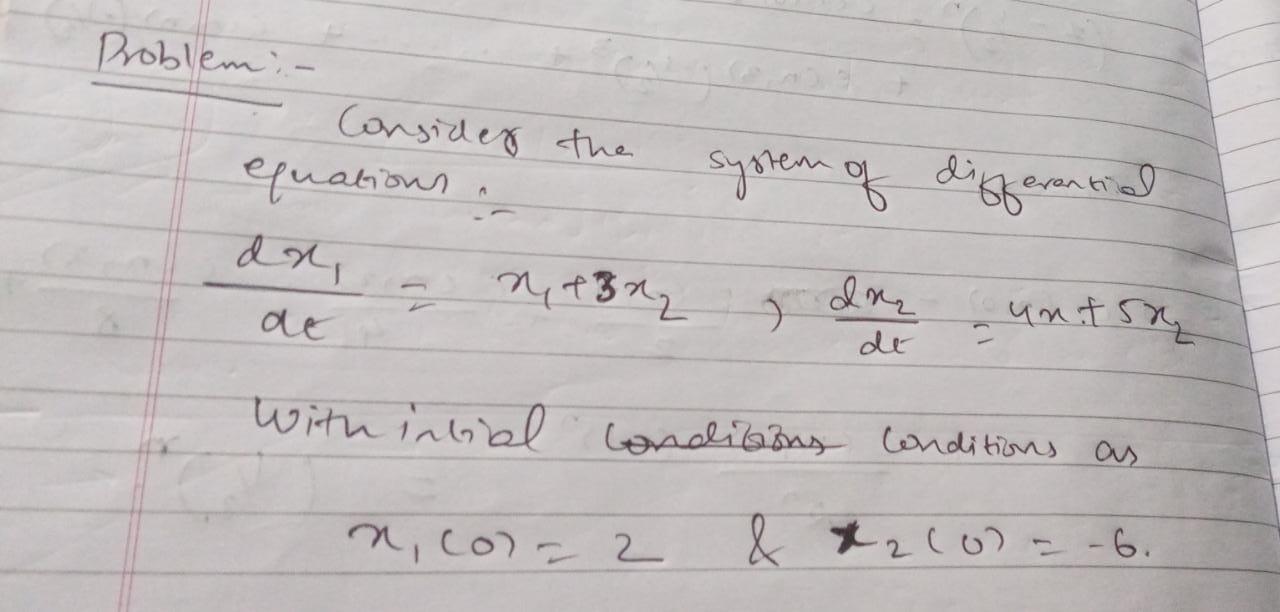
To perform eigenvalue decomposition, you first need to compute the eigenvalues and eigenvectors of a matrix A using a numerical method. The eigenvalues and eigenvectors are obtained from the characteristic equation |A - λI| = 0, where λ represents the eigenvalues and I is the identity matrix.
Step-by-Step Guide to Performing Eigenvalue Decomposition., How to compute eigenvectors from eigenvalues
The following steps are involved in performing eigenvalue decomposition:-
1. Compute the characteristic equation |A - λI| = 0 to obtain the eigenvalues of the matrix A.
2. Use the eigenvalues to compute the eigenvectors of the matrix A.
3. Normalize the eigenvectors using the formula v_i = v_i / ||v_i||, where ||v_i|| is the norm of the eigenvector.
4. The resulting eigenvectors are then the columns of the matrix V, and the eigenvalues are the diagonal elements of the matrix Λ.
Eigenvalue decomposition can be represented as A = VΛV^(-1), where V is the matrix of eigenvectors, Λ is the diagonal matrix of eigenvalues, and V^(-1) is the inverse of V.
Comparison of Eigenvalue Decomposition with Other Eigenvector Computation Methods.
Eigenvalue decomposition can be compared and contrasted with other eigenvector computation methods such as power iteration and Rayleigh quotient iteration. Both methods are widely used in various applications for computing eigenvectors from eigenvalues.| Method | Advantages | Disadvantages |
|---|---|---|
| Eigenvalue Decomposition | Computes eigenvectors from eigenvalues, accurate results, and widely used in various applications. | Requires large computational resources, slow for large matrices, and computationally intensive. |
| Power Iteration | Fast and efficient for computing dominant eigenvectors, widely used in various applications. | Not suitable for computing non-dominant eigenvectors, requires a good initial guess for convergence. |
| Rayleigh Quotient Iteration | Fast and efficient for computing multiple eigenvectors, widely used in various applications. | Not suitable for computing non-dominant eigenvectors, requires a good initial guess for convergence. |
Examples of Applications Where Eigenvalue Decomposition is Particularly Useful.
Eigenvalue decomposition has numerous applications in various fields, including:- Data Science: Eigenvalue decomposition is used in various data science applications such as dimensionality reduction, feature extraction, and clustering.
- Linear Algebra: Eigenvalue decomposition is used to compute eigenvectors from eigenvalues, and it is an essential tool in linear algebra.
- Image Processing: Eigenvalue decomposition is used in image processing to compute eigenvectors and eigenvalues of matrices representing images.
Computing Eigenvectors Can Be Complex and Time-Consuming for Large Matrices, Requiring the Use of Advanced Numerical Methods.
Computing eigenvectors from eigenvalues can be a daunting task, especially when dealing with large matrices. The complexity of the problem arises due to the need for precision in calculations and the potential for numerical instability. In such cases, the use of advanced numerical methods becomes essential to achieve accurate results.Differences Between Exact and Approximate Eigenvector Computation
Eigenvector computation can be approached in two ways: exact and approximate methods. While exact methods provide precise results, they can be computationally intensive and may not be feasible for large matrices. On the other hand, approximate methods offer a trade-off between accuracy and computational efficiency.- Exact methods, such as the QR algorithm and Jacobi algorithm, provide precise eigenvectors but are computationally expensive.
- Approximate methods, such as the power iteration and inverse iteration, offer a balance between accuracy and computational efficiency but may not provide exact results.
Using the QR Algorithm to Compute Eigenvectors
The QR algorithm is a popular method for computing eigenvectors due to its efficiency and accuracy. The algorithm involves the following steps:- Begin with an initial matrix A and perform QR decomposition to obtain Q and R.
- Compute the eigenvalues of R and sort them in descending order.
- Form the diagonal matrix D with the sorted eigenvalues and the unitary matrix V with the corresponding eigenvectors.
- Update the matrices A and R using the formula A ← V A V^H and R ← V R V^H.
- Repeat steps 2-4 until convergence.
Computational Complexity of Eigenvector Computation Methods
The computational complexity of eigenvector computation methods is a critical factor in determining their suitability for large matrices.| Method | Computational Complexity |
|---|---|
| QR Algorithm | O(n^3) |
| Powell's Iteration | O(n^2) |
| Jacobi Algorithm | O(n^3 log n) |
Visualizing eigenvectors and eigenvalues can be a useful tool for understanding the properties of a matrix.: How To Compute Eigenvectors From Eigenvalues
Visualizing eigenvectors and eigenvalues is a powerful technique for gaining insights into the behavior and properties of a matrix. By graphically representing the eigenvectors and eigenvalues, we can better understand the stability, convergence, and other characteristics of the system being modeled by the matrix. This visualization can greatly facilitate our understanding of complex systems and aid in making informed decisions.Relationship between eigenvectors and eigenvalues using a 2x2 matrix.
The relationship between eigenvectors and eigenvalues can be illustrated using a 2x2 matrix. Let's consider the following matrix:| a b |
| --- --- |
| c d |
The characteristic equation of this matrix is given by:
|A - λI| = 0
where A is the matrix, λ is the eigenvalue, and I is the identity matrix. Solving this equation, we can find the eigenvalues λ1 and λ2.
| a - λ b |
| --- --- --- |
| c d - λ |
Once we have the eigenvalues, we can find the corresponding eigenvectors v1 and v2 by solving the equation:
AV = λV
where V is the matrix of eigenvectors.
| Eigenvector | Eigenvalue |
|---|---|
v1 = [x1, x2] v2 = [y1, y2] |
λ1 λ2 |
Eigenvectors for visualizing matrix properties.
Eigenvectors can be used to visualize the properties of a matrix by plotting them in a graph. The direction and length of the eigenvectors can provide valuable information about the stability and convergence of the system.* Stability: If the eigenvalues have negative real parts, the eigenvectors will point in the direction of stability. This indicates that the system will return to its equilibrium state after a perturbation.
Limitations of using visualizations to understand eigenvectors and eigenvalues.
While visualizing eigenvectors and eigenvalues can provide valuable insights, there are some limitations to consider:* High-dimensional spaces: In high-dimensional spaces, it can be difficult to visualize the eigenvectors and eigenvalues accurately.
Closure
In conclusion, computing eigenvectors from eigenvalues is a complex but rewarding process that requires patience, persistence, and practice. With the right techniques and tools, you can master this mathematical skill and unlock new insights into the world of linear algebra. Remember, practice is key, so be sure to work through plenty of examples and exercises to deepen your understanding of this essential mathematical concept.
Helpful Answers
What is the difference between left eigenvectors and right eigenvectors?
Left eigenvectors are the transpose of right eigenvectors and are often denoted by the letter E. They are used to describe the behavior of matrices in a left-hand system, whereas right eigenvectors describe the behavior in a right-hand system.
How do I determine if a matrix is symmetric or non-symmetric?
A matrix is symmetric if it is equal to its transpose, and non-symmetric otherwise. To determine if a matrix is symmetric or non-symmetric, simply calculate its transpose and compare it to the original matrix.
What is the significance of diagonalization in eigenvector computation?
Diagonalization is a powerful technique used to compute eigenvectors from eigenvalues by representing a matrix in terms of its eigenvalues and eigenvectors. This can be particularly useful for large matrices, as it can simplify the computation process and provide more accurate results.
Leave a Comment
Comments are moderated before appearing. The data you submit is processed according to the Privacy Policy of guessthescore.