How to Make Line Graph with Excel in Minutes
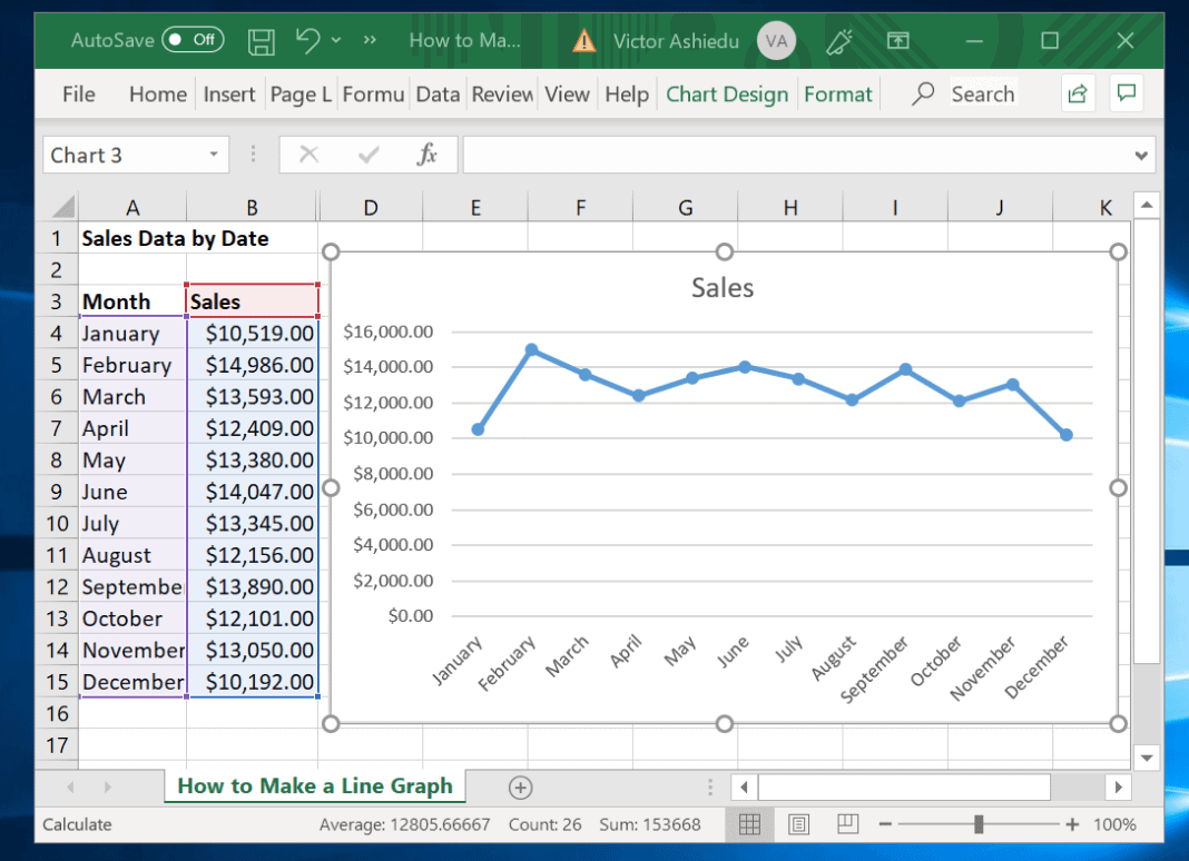
Table of Contents
- Creating a Basic Line Graph in Excel
- Selecting the Correct Chart Type
- Configuring the Graph's Appearance
- Using a Legend and Labeling Axes, How to make line graph with excel
- Example of Customizing the Graph's Appearance
- Example of Using a Legend and Labeling Axes
- Data Preparation for Creating a Line Graph
- Types of Data for Line Graphs
- Organizing Data for Analysis and Visualization
- Customizing Line Graphs in Excel
- Changing Colors and Line Styles
- Conditional Formatting
- Custom Charts
- Using Multiple Series in Line Graphs: How To Make Line Graph With Excel
- Creatng Separate Series
- Calculating and Displaying Moving Averages or Exponential Trends
- Example
- Advanced Line Graph Techniques in Excel
- Using Trendlines and Polynomial Regression
- Calculating Weighted Averages and Rolling Windows
- Customizing Graph Layouts and Resizing the Viewing Area
- Sharing and Exporting Line Graphs
- Copying to Clipboard and Printing
- If you want to share a line graph with others who may not have Excel, you can export it to a variety of image formats, including PNG, JPEG, and GIF. To do this, select the line graph and go to the "File" tab in the ribbon. Click on "Save As" and choose "Image" as the file type. You can then choose the desired image format and save the file. When exporting to an image format, you can also choose to include the chart in the file. To do this, select the line graph and go to the "File" tab in the ribbon. Click on "Save As" and choose "Image" as the file type. Under the "Options" tab, check the box next to "Include chart in file." This will include the chart in the image file. Troubleshooting and Optimizing Line Graphs When working with line graphs in Excel, you may encounter various issues that affect their appearance or functionality. Misaligned axes, misplaced data points, and poor performance are common problems that can arise when creating complex line graphs. In this section, we will explore troubleshooting and optimizing techniques to help you resolve these issues and create effective line graphs. Common Issues with Line Graphs
- Identifying and Resolving Issues
- Optimizing Graph Performance
- Case Study: Optimizing a Complex Dashboard
- Creating Responsive Line Graphs with HTML Tags
- Using HTML Tables with CSS Classes
- Applying Flexbox Properties
- Example: Applying Flexbox Properties to Arrrange Graph Components
- Last Recap
- Answers to Common Questions
With how to make line graph with Excel at the forefront, this article dives deep into creating an attractive line graph that showcases your data in the most effective way possible, covering the fundamentals and beyond.
This comprehensive guide will walk you through the process of creating a basic line graph, data preparation for line graphs, customizing line graphs, and even advanced techniques like using multiple series, trendlines, and responsive designs.
Creating a Basic Line Graph in Excel
To create a basic line graph in Excel, we need to follow a few simple steps. The first step is to insert data into a spreadsheet. This data can come from various sources, such as a database, a spreadsheet, or even manual input. Once we have our data, we can choose the correct chart type to create a basic line graph.
Selecting the Correct Chart Type
Selecting the correct chart type is a crucial step in creating a basic line graph in Excel. To do this, we need to follow these steps:
- First, select the range of cells that contain our data. We can do this by clicking and dragging the mouse over the cells.
- Next, go to the Insert tab in the ribbon and click on the Line Chart option.
- Select the type of line chart that we want to create. In this case, we want to create a basic line graph, so we select the "2-D Line" option.
- Click on the chart to select it and Excel will automatically create a basic line graph using the data that we selected.
Configuring the Graph's Appearance
Once we have created a basic line graph in Excel, we can configure its appearance to make it more informative and visually appealing. Here are the steps to configure the graph's appearance:
- First, we need to select the chart and go to the Design tab in the ribbon.
- Next, we can change the colors and styles of the chart by clicking on the "Change Colors" button in the "Chart Styles" group.
- We can also change the theme of the chart by clicking on the "Themes" dropdown menu in the "Chart Styles" group.
- We can further customize the graph's appearance by clicking on the "Quick Analysis" button in the "Data" group and selecting from the various options available.
- We can also add a title to the chart by clicking on the "Chart Title" option in the "Chart Elements" group.
Using a Legend and Labeling Axes, How to make line graph with excel
Using a legend and labeling axes is an important step in making our line graph more informative and easier to understand. Here are the steps to do this:
- First, we need to select the chart and go to the Chart Elements group in the ribbon.
- Next, we can add a legend to the chart by clicking on the "Legend" option and selecting the position where we want to place it.
- First, select the chart and go to the Chart Elements group in the ribbon.
- Next, click on the "Legend" option and select the position where you want to place it.
- Then, click on the "Axis Labels" option and select the labels that you want to add.
Time-series data
is ideal for showing trends over time. This can include sales figures, stock prices, or temperature readings over the course of a year or month. For example, visualizing quarterly sales data can reveal seasonal patterns and help businesses make informed decisions.categorical data
categorizes data into distinct groups. This can help illustrate progress or trends within these categories. For instance, comparing the performance of various sales teams can reveal which team is exceling and where improvement is needed.continuous data
can range from discrete values to very fine gradations. This type of data is often used to show how a particular quantity or factor changes over time or in response to something else. Examining the relationship between the number of customers served by a company and the number of products sold can help in identifying the ideal number of customers to focus on.Data sorting
is the process of arranging data in a particular order, such as alphabetically or chronologically. This helps identify patterns and trends more easily.Data cleaning
involves removing any errors, inaccuracies, or irrelevant data that could skew the results of analysis. This can include duplicates, missing values, or outliers that might affect the overall accuracy of the data.Data processing
may involve transforming or modifying the data in some way, such as converting it into a different format or calculating new values. This can include aggregating data, calculating rates or percentages, or filtering it to focus on specific aspects.- Change the color of a line by selecting the line and clicking on a new color in the "Format Data Point" pane.
- To change the line style, select the line and click on a new style in the "Format Data Point" pane.
- You can also customize the line style by choosing from a variety of options, including solid, dashed, and dotted lines.
- In addition to changing the color and line style, you can also customize the thickness of the line by dragging the "Line Width" slider in the "Format Data Point" pane.
- Add a shadow to a line by selecting the line and clicking on the "Shadow" button in the "Format Data Point" pane.
- You can also customize the shadow by adjusting the color, size, and position of the shadow.
- In addition to adding a shadow, you can also customize the appearance of a line graph by adding a border or a fill.
- To add a border or a fill, select the line and click on the "Border" or "Fill" button in the "Format Data Point" pane.
- To apply conditional formatting, select the line you want to customize by clicking on it.
- Click on the "Home" tab in the ribbon.
- Click on the "Conditional Formatting" button and select "New Rule" from the dropdown menu.
- Use the available options to specify the criteria for highlighting specific data points.
- To create a custom chart, select the data you want to use by clicking on it.
- Click on the "Insert" tab in the ribbon.
- Click on the " Chart" button and select "Line Chart" from the dropdown menu.
- Use the available options to customize the appearance of the chart.
- Select the entire dataset, including headers, and go to the "Insert" tab in the ribbon.
- Click on the "Line" option under the "Charts" group.
- Choose the line graph style you prefer and click on it.
- In the "Chart Elements" box, click the arrow next to "Series" and select "Edit Data" to create separate series.
- In the "Data Point" window, select the data range for each series and assign a label and color to each series.
- Click "OK" to apply the changes.
- Insert a new column next to your data, which will contain the moving average or exponential trend calculation.
- In the new column, use the following formula to calculate the moving average:
=AVERAGE(B2:B6)
for a 5-day moving average, where "B" represents the column with the data. - To calculate the exponential trend, use the
=EXP(INDEX(B:B,ROW(B:B)))
formula. - Select the entire dataset, including headers and the new column with the calculated values.
- Go to the "Insert" tab in the ribbon and click on the "Line" option under the "Charts" group.
- Choose the line graph style you prefer and click on it.
- In the "Chart Elements" box, click the arrow next to "Series" and select "Edit Data" to add the moving average or exponential trend series.
- In the "Data Point" window, select the data range for the moving average or exponential trend series and assign a label and color to it.
- Click "OK" to apply the changes.
- A trendline can be added to a line graph by clicking on the "Trendline" button in the "Chart Tools" tab.
- To create a polynomial regression, select the data range, go to the "Chart Tools" tab, and click on "Trendline" and then select "Polynomial" from the dropdown menu.
- You can adjust the order of the polynomial equation by selecting the "Options" button and then adjusting the "Order" slider.
- To calculate a weighted average in Excel, use the formulas =AVERAGE(range, weight1, weight2, ...) where weight1, weight2, etc. are the weights assigned to each data point.
- To create a rolling window analysis, use the formulas =AVERAGE(range1, range2, ...) where range1, range2, etc. are the data ranges for the specified period.
- To customize the graph layout, click on the "Chart Tools" tab and select the "Layout" options.
- To resize the viewing area, click on the chart and drag the borders to adjust the size and position.
- Misaligned Axes:
- Placed Data Points:
- Poor Performance:
- Check Axis Labels and Tick Marks: Make sure axis labels and tick marks are consistent and easy to read. Use the same label and tick mark formatting throughout the graph.
- Adjust Data Layout: Experiment with different data layouts to ensure data points are aligned correctly. Use grouping or stacking to organize data points and make them easier to read.
- Optimize Performance: Limit the number of data points, data series, and graph elements. Simplify your graph by removing unnecessary features and focusing on the most critical information.
- Adjust Refresh Rates: Adjust the data refresh rate to ensure the graph updates quickly. A slow refresh rate can cause the graph to freeze or stall.
- Caching: Enable caching to store frequently used data and reduce the load on the graph. Caching can significantly improve graph performance and rendering speed.
li>We can also label the axes by clicking on the "Axis Labels" option and selecting the labels that we want to add.
Example of using a legend: Let's say we have a line graph that shows the sales of different products over time. We can add a legend to the chart to show which product each line represents. This makes it easier for the reader to understand the data and make informed decisions.
Example of Customizing the Graph's Appearance
Here's an example of customizing the graph's appearance:
| Step | Description |
|---|---|
| 1 | Change the colors of the chart to blue and green. |
| 2 | Change the theme of the chart to a modern theme. |
| 3 | Remove the gridlines from the chart. |
| 4 | Add a title to the chart that says "Sales of Different Products Over Time". |
Example of Using a Legend and Labeling Axes
Here's an example of using a legend and labeling axes:
Let's say we have a line graph that shows the sales of different products over time. We can add a legend to the chart to show which product each line represents. We can also label the axes to show the units of measurement for the data.
Data Preparation for Creating a Line Graph
For a line graph to convey meaningful and effective insights, careful data preparation is essential. This involves selecting and organizing data points, ensuring accurate labeling, and choosing the right type of data to represent.
To create a compelling line graph, it's crucial to identify the key elements necessary for analysis and visualization. This includes data points, which are the individual values that make up the graph; the x-axis, which typically represents time or categories; and the y-axis, which represents the values being measured. Labeling these elements accurately helps convey the story behind the data.
Types of Data for Line Graphs
Line graphs are versatile and can represent various types of data, including time-series, categorical, and continuous data. Understanding the differences between these types helps in selecting the right data for visualization.
Organizing Data for Analysis and Visualization
Organizing data in a structured manner is crucial for creating effective line graphs. This involves ensuring that data is properly sorted, cleaned, and processed before being used for analysis.
Customizing Line Graphs in Excel
Line graphs are a valuable tool for showcasing trends and patterns in data, but they can be even more effective when customized to highlight the most important information. In this section, we'll explore the various options available for modifying the appearance of a line graph, including changing colors, adding shadows, and adjusting line styles.
Changing Colors and Line Styles
When it comes to customizing line graphs, one of the most effective ways to draw attention to specific data points is by changing the colors and line styles. This can be particularly useful when comparing multiple sets of data or highlighting specific trends.
To change the color and line style of a line graph, follow these steps:
1. Select the line you want to customize by clicking on it.
2. Click on the "Format" tab in the ribbon.
3. Select "Format Data Point" from the dropdown menu.
4. Use the available options to customize the color and line style of the line.
In addition to changing the color and line style, you can also customize the appearance of a line graph by adding shadows and other effects. This can help draw attention to specific data points and create a more visually appealing graph.
To add a shadow or other effects to a line graph, follow these steps:
1. Select the line you want to customize by clicking on it.
2. Click on the "Format" tab in the ribbon.
3. Select "Format Data Point" from the dropdown menu.
4. Use the available options to customize the shadow, border, or fill of the line.
Conditional Formatting
Conditional formatting is a powerful tool that allows you to highlight specific data points on a line graph based on certain criteria. This can be particularly useful when comparing multiple sets of data or highlighting specific trends.
To apply conditional formatting to a line graph, follow these steps:
1. Select the line you want to customize by clicking on it.
2. Click on the "Home" tab in the ribbon.
3. Click on the "Conditional Formatting" button and select "New Rule" from the dropdown menu.
4. Use the available options to specify the criteria for highlighting specific data points.
Custom Charts
Custom charts are a powerful tool that allows you to create custom charts based on calculated fields and user-defined formulas. This can be particularly useful when creating complex charts or visualizations.
To create a custom chart, follow these steps:
1. Select the data you want to use by clicking on it.
2. Click on the "Insert" tab in the ribbon.
3. Click on the " Chart" button and select "Line Chart" from the dropdown menu.
4. Use the available options to customize the appearance of the chart.
Using Multiple Series in Line Graphs: How To Make Line Graph With Excel
Visualizing multiple data sets or time intervals on a single line graph is essential in Excel when you need to compare trends or patterns within various categories, such as different months, product lines, or geographic regions. This feature allows you to analyze the relationships between data series in a concise and informative manner.
Creatng Separate Series
To create separate series using various data points, labels, and colors in a line graph, follow these steps:
By using separate series, you can easily identify and compare trends within different categories, making it easier to draw conclusions and make informed decisions.
Calculating and Displaying Moving Averages or Exponential Trends
To calculate and display moving averages or exponential trends in a line graph, follow these steps:
The use of moving averages and exponential trends can help you identify patterns and trends in your data that may not be immediately apparent, providing valuable insights for decision-making and analysis.
Example
Suppose you have a dataset with monthly sales figures for three different product lines. You want to create a line graph that displays the sales trend for each product line over a period of 12 months. To do this, follow the steps Artikeld above.
Advanced Line Graph Techniques in Excel
Advanced line graph techniques in Excel are essential for analyzing complex data patterns, making predictions, and gaining insights. By mastering these techniques, you can create informative and visually appealing line graphs that help you make informed decisions. In this section, we will explore some advanced techniques, including the use of trendlines, polynomial regression, weighted averages, and customized graph layouts.
Using Trendlines and Polynomial Regression
Trendlines and polynomial regression are powerful tools for analyzing and visualizing complex data patterns. A trendline is a line that best fits the data points, showing the overall direction and trend of the data. Polynomial regression is a type of trendline that uses a polynomial equation to fit the data, allowing for more complex relationships between variables.
"The goal of trendline analysis is to identify the overall direction and trend of the data, rather than individual data points."
Calculating Weighted Averages and Rolling Windows
Weighted averages and rolling windows are useful techniques for analyzing time-series data. A weighted average gives more importance to recent data points, while a rolling window analysis looks at a fixed number of data points over a specified period.
"Weighted averages and rolling windows are useful for analyzing time-series data, as they give more importance to recent data points and help to smooth out noise."
Customizing Graph Layouts and Resizing the Viewing Area
Customizing graph layouts and resizing the viewing area are essential for improving data clarity and making the graph more readable. By adjusting the layout and scale of the graph, you can highlight important trends and relationships.
"A well-designed graph layout and viewing area can make a huge difference in data interpretation and decision-making."
Sharing and Exporting Line Graphs
When you've finished creating your line graph in Excel, you'll likely want to share it with others or incorporate it into reports, presentations, or external websites. Excel provides several methods for saving and sharing line graphs, each with its own advantages. In this section, we'll explore the various ways to share and export line graphs, from copying to clipboard to exporting to image formats.
Copying to Clipboard and Printing
One of the simplest ways to share a line graph is to copy it to the clipboard and paste it into another application. To do this, select the line graph and go to the "Home" tab in the Excel ribbon. Click on the "Copy" button in the "Clipboard" group, or press Ctrl+C on your keyboard. You can then paste the graph into another application, such as a word processor or presentation software.
You can also print a line graph directly from Excel. To do this, select the graph and go to the "File" tab in the ribbon. Click on "Print" and choose your desired print options, such as printer, page layout, and paper size.
If you want to share a line graph with others who may not have Excel, you can export it to a variety of image formats, including PNG, JPEG, and GIF. To do this, select the line graph and go to the "File" tab in the ribbon. Click on "Save As" and choose "Image" as the file type. You can then choose the desired image format and save the file.
When exporting to an image format, you can also choose to include the chart in the file. To do this, select the line graph and go to the "File" tab in the ribbon. Click on "Save As" and choose "Image" as the file type. Under the "Options" tab, check the box next to "Include chart in file." This will include the chart in the image file.
Troubleshooting and Optimizing Line Graphs
When working with line graphs in Excel, you may encounter various issues that affect their appearance or functionality. Misaligned axes, misplaced data points, and poor performance are common problems that can arise when creating complex line graphs. In this section, we will explore troubleshooting and optimizing techniques to help you resolve these issues and create effective line graphs.Common Issues with Line Graphs
Several common issues can affect the appearance or functionality of line graphs. Understanding these problems will help you address them effectively.Misaligned axes can make your line graph difficult to read. Axis labels and tick marks may appear inconsistent or confusing.
Placed data points can affect the overall appearance of a line graph. Misaligned data points may look cluttered or messy, making it hard to read.
Poor performance can make a line graph slow to render or cause it to freeze when zooming in or out.
Identifying and Resolving Issues
To resolve these issues, it's essential to understand the root cause of the problem. Here are some step-by-step guides to help you troubleshoot and optimize your line graphs:Optimizing Graph Performance
Optimizing graph performance is crucial to ensure your line graph renders quickly and efficiently. Here are some step-by-step guides to help you optimize your graph performance:Case Study: Optimizing a Complex Dashboard
In a real-world scenario, a financial analyst created a complex dashboard with multiple line graphs and data series. However, the graph took several seconds to render, causing frustration for users. By applying optimization techniques, the analyst simplified the graph, limited the number of data points, and enabled caching. As a result, the graph rendered quickly and efficiently, improving user experience and productivity.Ongoing maintenance and optimization are crucial to ensure your line graphs remain effective and efficient.
Leave a Comment
Comments are moderated before appearing. The data you submit is processed according to the Privacy Policy of guessthescore.